The Tennis Court Problem (TCP)

Posted on 26. July 20236. December 2023 by Fabian Leuthold

I owe this task to Ruedi, a regular tennis player. The Tennis Court Problem (TCP) is about the following task. At the beginning of outdoor tennis, the court lines must always be cleaned first. The sweeping set is often placed in one of two typical locations, usually either on one side of the net or in a corner. I owe this task to a relative, who is a regular tennis player.

In this post we will first describe the problem, then show a well explained way how to tacke the problem with integer linear programming (ILP) and finally implement the solution in python using the SCIP or GUROBI solver.

Thinking of the problem mentioned following questions come to mind:

Question 1: In what order should each section of the court lines be cleaned so that the distance traveled is as short as possible if the cleaning tour is to start and end at the location of the sweeping set?
Question 2: Is a particular placement of the sweeping set (at the net or at the corner) preferable for the resulting tour?

Problem

The task is to find the shortest route visiting all sections of the court lines at least once, starting and ending at the location of the sweeping set.

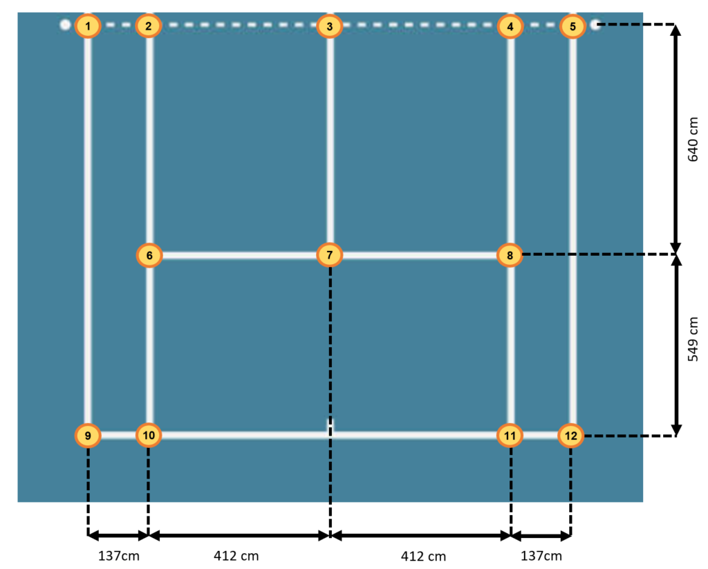
The total length of the court lines to be cleaned is 7318 cm:

$l_{tot} = 4 \cdot (549 + 640) + 640 + 2 \cdot (2 \cdot 412 + 137) = 7318$

We can model this task as a graph problem consisting of vertices and edges. Graph theory can help us to determine, that based on the degrees of the vertices, we know we cannot find a closed tour connecting all the line segments to be cleaned exactly once. This would be an Eulerian cycle, but it exists only in connected graphs where all vertices have an even degree.

One could try to use a tree search based heuristic approach to determine possible ways traversing the graph from the starting vertice, while trying to keep track of unwanted cycling.

The simplest approach however is to find an integer linear program, and that’s the approach we want to take.

The Model

We want to find a model which solves our problem described. In the following sections I describe how the model is built. For german readers please obtain the LaTeX version here. Before we start modeling it often helps to think of the answer we want to get from the model: We want to know, which line segment we have to visit (clean) in sequence in such a way that

the total distance traveled is minimized (the distance to clean is constant)
the tour must start and end at a defined location (where the sweeping set is)

Decision Variable(s)

Firstly, the decision variable must be able to arrange the vertices 1-12 in a sequence. Since the model must be linear, we need to have the sequence information encoded in the idices. We thus need at least two indices. However, since the model must allow to distinguish multiple visits in the same vertice, we need to introduce another index to uniquely ‘name’ the steps in the sequence:

$X_{ijk}$ : Binary decision variable indicating whether in the $i$ -th step the court line segment between vertice $j$ and $k$ is processed (=1) or not (=0).

Indices and Sets

The following indices and sets provide the means to further characterize the variables and parameters of the ILP:

$I$ : The set of individual steps to walk the line network: $I=\{1,...,n\}.$
$i \in I}$ : The $i$ -th step from the set of steps $I$ necessary to traverse the line net from start to end.
$N$ : The set of vertices of the graph network describing the tennis court $N=\{1,...,12\}$ .
$(j,k) \in N$ : A single line segment bounded by the adjacent vertices $j$ and $k$ .

Parameters

To find out, what parameters we need, we usually just start modeling the constraints and repeatedly add the parameters we need to write down the constraints step by step. However, here comes the complete list as it turned out to meet the needs after the modeling process:

$n$ : Number of total steps in the sequence of line segments to stepped trhough. This parameter is determined heuristically in order to find the minimum number of necessary segments that have to be run in order to clean the entire line network and return to the starting point. The heuristic starts at $n = |N|$ and increases n by 1 after each failed attempt to solve the model until finally the model is feasible and the optimal solution can be found.
$W_{jk}$ : Binary parameter indicating whether it is possible to go from vertice $j$ to vertice $k$ (=1), 0 otherwise.
$M_{jk}$ : Binary parameter indicating whether the line segment from vertice $j$ to $k$ must be cleaned (=1), 0 otherwise.
$D_{jk}$ : Real-valued parameter indicating how long the line segment between vertice $j$ and $k$ is (e.g. in cm).
$s$ : Index of the starting vertice $s \in N$ , indicating the location of the sweeping set where the cleaning tour has to start and end.

Constraints

Now here come the constraints. In this design step we try to formulate the requirements the decision variables have to meet in order for the model to represent our model we have in mind. Usually it is in this step, where we realize, that the choice for the decision variable was unfavourable. We then take a step back and try to express the solution to our problem in another fashion, then come back and again try to write down the constraints.

C1: Allow only allowed successor vertices
$\forall (j,k) \in (N \times N): \sum_i X_{ijk} \leq n \cdot W_{jk}$
This constraint ensures that only allowed successor vertices are accepted.
C2: Process exactly one lines segment in each step
$\forall i \in \{1..n\}: \sum_{(j,k)} X_{ijk} = 1$
This constraint ensures that only exactly one path segment may be traversed in a given direction in each step.
C3: Clean all line segments to be cleaned
$\forall (j,k) \in (N \times N): \sum_{i} X_{ijk} + X_{ikj} >= M_{jk}$
This constraint ensures that – if the path segment between vertices $i$ and $j$ needs to be cleaned, that it is traversed at least once in any direction.
C4: Path starts at start vertice
$\sum_k X_{1sk} = 1$
This constraint ensures that the first step is to go from the start vertice to another (due to C1 allowable, reachable) vertice.
C5: Path ends at start vertice
$\sum_k X_{nks} = 1$
This constraint ensures that the last step is to go from a (due to C1 allowable, reachable) vertice to the start vertice.
C6: Contiguous path
$\forall (i, k) \in ({1,...,n-1\}, k \in N): \sum_j X_{ijk} = \sum_j X_{i+1,kj}$
This constraint ensures that the subpaths of the sequence represent a contiguous path. Note that the index i does not cover the last node.

Objective Function

The objective function needs to minimize the distance to be run to clean all the necessary subsections. Here we make use of the parameter D, telling the distance we have to walk to connect the line segments between two adjacent vertices.

$min \quad \sum_{ijk} X_{ijk} \cdot D_{jk}$

Model Validation

One very important step is the validation step. Validation can be done in different phases of the modeling process. The first two steps are considered in the modeling phase, where as the last one is performed after implementation:

Perform an index check: Make sure, there are no free indices in the equations
Logical checks: Does the model allow solutions which should not be allowed or does it supress valid solutions?
Application/solution check: Let the model solve problem instances and check, whether the delivered solutions make sense

Wheres index inconsistencies are usually detected by the development environment on design time, we typically detect design flaws when we first see the results or the ‘missing’ results (if the model keeps turning out infeasible). Sometimes we immideately realize, what we missed. Sometimes we don’t. Then we have to doubleckeck the value range of the variables, deactivate single constraints, modify with the objective function to track down the issue.

The Solution

The model provides the same optimum for both broom locations. Below is the visualization of one optimal (minimum) solution each.

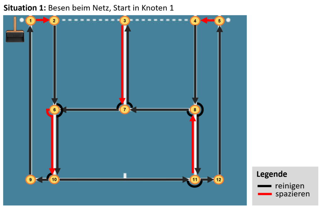
**Variant 1:** Optimal solution for sweeping set placed at the border of the net

**Variant 2:** Optimal solution for sweeping set placed in the corner of the court

In both cases, the total distance covered is identical. It is calculated from the sum of the sections to be cleaned (black) and the walked sections where cleaning is not performed (red):

$l_{opt} = 7318 + 2 \cdot 549 + 640 + 2 \cdot 137 = 9330$

In other words: We have to walk at least 93.3 meters if we want to clean the court lines from one half of the court. By choosing different locations for the sweeping set, we can check if different placements have a positive effect on the optimum found. However, this is not the case. The minimum required distance of 93.3 m cannot be undercut. It is open source under GPLv3 license.

The Source

In the following I present the solution modeled in python using Google OR-Tools together with the ‘SCIP’ solver. For bigger problems I usually use GUROBI, however, for such small simple problems other solvers can be used as well. Which solver you want to use can be configured in the variable ”solver_name” of the function solve_ILP. The same source code can be obtained here from my github account.

from ortools.linear_solver import pywraplp
import numpy as np


def solve_ILP(W, M, D, N, s, n):
    """
    Erstellung des ILP Modells, aufrufen des Solvers und Rückgabe der Lösung

    :param W: Angabe, welche Knoten (direkt) voneinander erreichbar sind
    :param M: Angabe, ob Wegstück zu reinigen ist
    :param D: Distanzen zwischen den Knoten
    :param N: Menge aller Knoten
    :param s: Index des Startknotens (0-based)
    :param n: Länge der Wegstücke
    :return:
    """

    # Create the model.
    # solver_name = 'GUROBI_MIP'
    solver_name = 'SCIP'
    model = pywraplp.Solver.CreateSolver(solver_name)
    model.EnableOutput()

    # Menge aller Lauf-Schritte definieren
    STEPS = list(range(n))
    STEPS_WO_LAST = list(range(n - 1))

    # Erzeugung der Entscheidungsvariablen X
    X = {}
    for i in STEPS:
        for j in N:
            for k in N:
                X[(i, j, k)] = model.BoolVar('task_i%ij%ik%i' % (i, j, k))

    # constraint 1: Nur zulässige Nachfolgeknoten erlauben
    for j in N:
        for k in N:
            model.Add(sum(X[(i, j, k)] for i in STEPS) <= n * W[j][k])

    # constraint 2: In jedem Schritt exakt ein Wegstück ablaufen
    for i in STEPS:
        model.Add(sum(X[(i, j, k)] for j in N for k in N) == 1)

    # constraint 3: Alle zu reinigenden Wegstücke reinigen
    for j in N:
        for k in N:
            model.Add(sum(X[(i, j, k)] + X[(i, k, j)] for i in STEPS) >= M[j][k])

    # constraint 4: Anfangspunkt beim Startknoten
    model.Add(sum(X[(0, s, k)] for k in N) == 1)

    # constraint 5: Endpunkt beim Startknoten
    model.Add(sum(X[(n - 1, k, s)] for k in N) == 1)

    # constraint 6: Zusammenhängender Pfad
    for i in STEPS_WO_LAST:
        for k in N:
            model.Add(sum(X[(i, j, k)] for j in N) == sum(X[(i+1, k, j)] for j in N))

    # Zielfunktion
    model.Minimize(sum(X[(i, j, k)] * D[j][k] for i in STEPS for j in N for k in N))

    status = model.Solve()
    if status == pywraplp.Solver.OPTIMAL:
        model_solved = True
        ret_x = convert_X(X, len(STEPS), len(N), len(N))
        objective_value = model.Objective().Value()
    else:
        model_solved = False
        ret_x = None
        objective_value = None

    return model_solved, ret_x, objective_value

def convert_X(X, dim_i, dim_j, dim_k):
    """
    Konvertiert die 3d Google OR-Tools Solution-Variable X_ijk in eine brauchbare Variable

    :param X: Google OR-Tools 3d-solution Variable
    """

    ret_X = np.zeros(shape=(dim_i, dim_j, dim_k), dtype=np.int8)
    for i in range(0, dim_i):
        for j in range(0, dim_j):
            for k in range(0, dim_k):
                ret_X[i, j, k] = X[(i, j, k)].solution_value()

    return ret_X


def find_needle(X, i, dim_jk):
    """
    finds the location (j,k), where a boolean is set in line i
    :param X:
    :param i: line i
    :param dim_jk: the size of the sub-field
    :return: j, k
    """
    for j in range(dim_jk):
        for k in range(dim_jk):
            if X[i, j, k] == 1:
                return j, k
            elif X[i, k, j] == 1:
                return k, j
    return None, None

if __name__ == '__main__':
    # W_jk:  Binärer Parameter der angibt, ob von Knoten  zum Knoten  gegangen werden kann (=1), 0 sonst.
    #     1  2  3  4  5  6  7  8  9  10 11 12
    W = [[0, 1, 0, 0, 0, 0, 0, 0, 1, 0, 0, 0],  # 1
         [1, 0, 1, 0, 0, 1, 0, 0, 0, 0, 0, 0],  # 2
         [0, 1, 0, 1, 0, 0, 1, 0, 0, 0, 0, 0],  # 3
         [0, 0, 1, 0, 1, 0, 0, 1, 0, 0, 0, 0],  # 4
         [0, 0, 0, 1, 0, 0, 0, 0, 0, 0, 0, 1],  # 5
         [0, 1, 0, 0, 0, 0, 1, 0, 0, 1, 0, 0],  # 6
         [0, 0, 1, 0, 0, 1, 0, 1, 0, 0, 0, 0],  # 7
         [0, 0, 0, 1, 0, 0, 1, 0, 0, 0, 1, 0],  # 8
         [1, 0, 0, 0, 0, 0, 0, 0, 0, 1, 0, 0],  # 9
         [0, 0, 0, 0, 0, 1, 0, 0, 1, 0, 1, 0],  # 10
         [0, 0, 0, 0, 0, 0, 0, 1, 0, 1, 0, 1],  # 11
         [0, 0, 0, 0, 1, 0, 0, 0, 0, 0, 1, 0]]  # 12
    # M_jk: Binärer Parameter der angibt, ob das Wegstück von Knoten  zum Knoten  gereinigt werden muss (=1), 0 sonst.
    # Matrix ist symmetrisch.
    #     1  2  3  4  5  6  7  8  9  10 11 12
    M = [[0, 0, 0, 0, 0, 0, 0, 0, 1, 0, 0, 0],  # 1
         [0, 0, 0, 0, 0, 1, 0, 0, 0, 0, 0, 0],  # 2
         [0, 0, 0, 0, 0, 0, 1, 0, 0, 0, 0, 0],  # 3
         [0, 0, 0, 0, 0, 0, 0, 1, 0, 0, 0, 0],  # 4
         [0, 0, 0, 0, 0, 0, 0, 0, 0, 0, 0, 1],  # 5
         [0, 1, 0, 0, 0, 0, 1, 0, 0, 1, 0, 0],  # 6
         [0, 0, 1, 0, 0, 1, 0, 1, 0, 0, 0, 0],  # 7
         [0, 0, 0, 1, 0, 0, 1, 0, 0, 0, 1, 0],  # 8
         [1, 0, 0, 0, 0, 0, 0, 0, 0, 1, 0, 0],  # 9
         [0, 0, 0, 0, 0, 1, 0, 0, 1, 0, 1, 0],  # 10
         [0, 0, 0, 0, 0, 0, 0, 1, 0, 1, 0, 1],  # 11
         [0, 0, 0, 0, 1, 0, 0, 0, 0, 0, 1, 0]]  # 12

    # D_jk: Reellwertiger Parameter der angibt, wie lange das Wegstück zwischen den Knoten  zum Knoten  ist (in cm).
    # Quelle: https://tennis-uni.com/tennisplatz-tennisfeld/
    # Länge aller Linien: (549+640)*4+640+824*2+137*2+823=8141
    # Länge aller Linien: 4*(549+640)+640+2*(2*412+137)
    #     1     2    3    4    5    6    7    8    9    10   11   12
    D = [[000, 137, 000, 000, 000, 000, 000, 000, 1189, 000, 000, 000],  # 1
         [137, 000, 412, 000, 000, 640, 000, 000, 000, 000, 000, 000],  # 2
         [000, 412, 000, 412, 000, 000, 640, 000, 000, 000, 000, 000],  # 3
         [000, 000, 412, 000, 137, 000, 000, 640, 000, 000, 000, 000],  # 4
         [000, 000, 000, 137, 000, 000, 000, 000, 000, 000, 000, 1189],  # 5
         [000, 640, 000, 000, 000, 000, 412, 000, 000, 549, 000, 000],  # 6
         [000, 000, 640, 000, 000, 412, 000, 412, 000, 000, 000, 000],  # 7
         [000, 000, 000, 640, 000, 000, 412, 000, 000, 000, 549, 000],  # 8
         [1189, 000, 000, 000, 000, 000, 000, 000, 000, 137, 000, 000],  # 9
         [000, 000, 000, 000, 000, 549, 000, 000, 137, 000, 824, 000],  # 10
         [000, 000, 000, 000, 000, 000, 000, 549, 000, 824, 000, 137],  # 11
         [000, 000, 000, 000, 1189, 000, 000, 000, 000, 000, 137, 000]]  # 12

    solved = False
    anz_knoten = 12
    N = list(range(anz_knoten))
    # Startknoten Index s (0-based)
    s = 0
    n = len(N)
    n_max = 2 * len(N)

    while not solved and n <= n_max:
        solved, X, obj_val = solve_ILP(W, M, D, N, s, n)
        if not solved:
            print("Shit... No solution found for path with length {} Next try.".format(n))
        n = n + 1

    if not solved:
        print("Keine Lösung gefunden :(")
    else:
        print("Lösung gefunden! :)")
        for i in range(n - 1):
            j,k = find_needle(X, i, len(N))
            print("In schritt {} gehe ich von Knoten {} nach Knoten {}.".format(i+1, j+1, k+1))