Vertex Coloring using ILP

Posted on 7. August 20237. August 2023 by Fabian Leuthold

In this post I’ll show you how to solve the vertex coloring problem to optimality using linear programming. Since the problem is NP-complete, there is no algorithm which can solve any problem instance in deterministic polynomial time. In a former post, I used constraint programming to find an optimal (minimal) vertex coloring.

A popular greedy heuristic approach for vertex coloring is demonstrated in this movie here by Rhyd Lewis. It demonstrates a simple approach to color vertices of a given graph.

Here, we will first develop an ILP (Integer Linear Program) to solve the problem, as it is presente. Here we will first develop an ILP (Integer Linear Program) to solve the problem. The information and inspiration for this post comes from the lecture notes of Prof. Dr. Petra Mutzel, University of Bonn. In her notes you can find many further and deeper considerations to improve the model introduced here and to break symmetries in the model.

In a second step I’ll demonstrate, how to translate the model into python code to solve the vertex coloring problem for “any” given graph (“any” in quotation marks: The limitation here is the problem-size causing combinatorial explosion. Today, top ILP solvers can easily handle up to 1 mio decision variables).

The Model

Given a Graph $G$ , consisting of a set of vertices $V$ and Edges $E$ . A vertice coloring is valid or admissible if any two adjacent vertices do not have the same color. If a graph is colorable, there is a smallest number (the ghrah’s chromatic number, usually denoted by $\chi(G)$ ) such that the graph is vertice colorable.

A graph with n nodes it is certainly n colorable. Our model should assign one color $c$ out of $C=\{1, ..., n\}$ to each vertex $v$ in such a way, that no adjacent nodes have the same color and the number of colors needed is minimized.

Decision Variable(s)

Since we want to assign a color to each vertex, it makes sense to choose a decision variable with two indices: One for identifying the vertex and one for the color:

$X_{vc}$ : Binary decision variable, indicating whether vertex $v$ is colored with color $c$ (=1), or not (=0).

At the latest when we want to formulate the objective function, we realize that we still need an auxiliary variable. Our goal is to minimize the number of assigned colors. I.e. we would like to have a variable that tells us which of the colors $c \in C$ haven been assigned in the solution:

$W_c$ : Binary decision variable, indicating whether color $c$ was assigned in the solution (=1), or not (=0).

Indices and Sets

The following indices and sets provide the means to further characterize the variables and parameters of the ILP:

$v \in V$ : A specific vertex of the set of the graph’s vertices
$e \in E$ : An edge of the graph
$c \in C$ : The ID of color $c \in C=\{1, ..., n\}$

Constraints

We have already learned about a contraint in the formulation of the problem. It describes which condition must be fulfilled for a coloring to be valid. In addition, we must ensure that each node is assigned exactly one color.

C1: Assign exactly one color to each vertices
$\forall v \in V: sum_{c\in C} X_{v,c} = 1$
This constraint makes sure, that for any specific vertice exactly one color is assigned.
C2: Adjacent vertices have different colors
$\forall (u, v) \in E, c \in C: X_{uc} + X_{vc} \le W_c$
This constraint makes sure, that for any pair of two vertices $(u, v)$ connected by an edge $e \in E$ and any defined color $c$ no more than one of both vertices is colored in color $c$ . Simulatneously it takes care of defining the auxiliary variable $W_c$ .

Objective Function

The objective function needs to minimize the colors used to color the vertices. Thanks to the auxiliary variable defined above, this is now a simple task:

$min \quad \sum_{c \in C} U_c$

The Solution

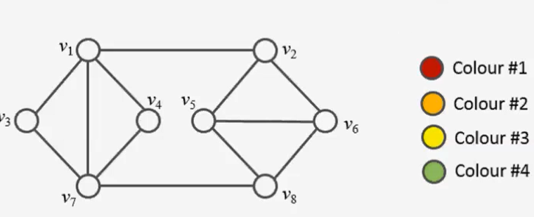
The source not only shows the implementation of the ILP but also demonstrates the difference between a greedy coloring heuristic and an exact solution approach. The task below is first colored using the largest_first greedy coloring heuristic of the networkX library, then the same task is colored using the ILP.

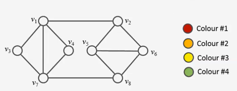
A sample graph for our coloring ILP [Source: youtube clip from Dr. Rhyd Lewis]

In the script below I first construct the graph shown above defining an adjacency list. Then the graph is colored using the largest_first greedy coloring heuristic of the networkX library. This gives the following result:

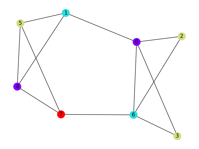
As we can see, the heuristic returns a coloring that requires four colors. If we let the ILP color the same graph, we get the following result:

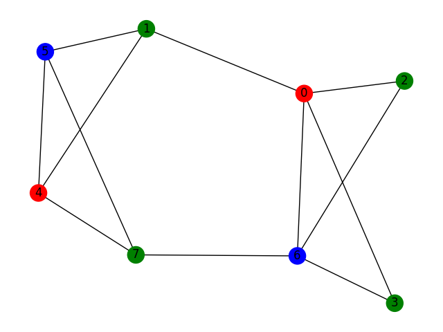
Graph colored using our ILP model from above

So we see that the ILP has done a better job. It has found the minimal coloring requiring only three colors.

In the movie mentioned above from Mr. Dr. Rhyd Lewis he explains, how the greedy coloring heuristic works. There it is also nicely shown that the heuristic can find the optimal coloring depending on the initial situation.

The Source

In the following I present the solution modeled in python using Google OR-Tools together with the ‘SCIP’ solver. For bigger problems I usually use GUROBI, however, for such small and simple problems other solvers can be used as well. Which solver you want to use can be configured in the variable ”solver_name” of the function solve_ILP. The same source code can be obtained here from my github account.

from ortools.linear_solver import pywraplp
import numpy as np
import networkx as nx
import itertools
import matplotlib.pyplot as plt


def solve_ILP(adj_list):
    """
    Creation of the Assignment model, based on Lecture slides of Mr. Dr. Petra Mutzel, University Bonn

    https://www.or.uni-bonn.de/~held/hausdorff_school_22/slides/GraphColoringFormulations.pdf

    :param W: Angabe, welche Knoten (direkt) voneinander erreichbar sind
    :param M: Angabe, ob Wegstück zu reinigen ist
    :param D: Distanzen zwischen den Knoten
    :param N: Menge aller Knoten
    :param s: Index des Startknotens (0-based)
    :param n: Länge der Wegstücke
    :return:
    """

    # Create the model.
    solver_name = 'SCIP'
    model = pywraplp.Solver.CreateSolver(solver_name)
    model.EnableOutput()

    # determine the number of nodes
    dim = len(set(itertools.chain.from_iterable(adj_list)))
    # set of nodes
    V = list(range(dim))
    # set of colors
    I = V

    # create decision vars
    X = {}
    W = {}
    for v in V:
        for i in I:
            X[(v, i)] = model.BoolVar('task_v%ii%i' % (v, i))
    for i in I:
        W[i] = model.BoolVar('task_i%i' % i)

    # constraint 1: every node needs to get assigned one color
    for v in V:
        model.Add(sum(X[(v, i)] for i in I) == 1)

    # constraint 2: neighboring nodes not same color
    for i in I:
        for u, v in adj_list:
            model.Add(X[(u, i)] + X[(v, i)] <= W[i])

    # Zielfunktion
    model.Minimize(sum(W[i] for i in I))

    status = model.Solve()
    if status == pywraplp.Solver.OPTIMAL:
        model_solved = True
        ret_x = convert_X(X, dim)
        objective_value = model.Objective().Value()
    else:
        model_solved = False
        ret_x = None
        objective_value = None

    return model_solved, ret_x, objective_value


def convert_X(X, dim):
    """
    converts the 2d Google OR-Tools Solution-Variable X_ij to an np.array
    :param X: Google OR-Tools 2d-solution Variable
    """

    ret_X = np.zeros(shape=(dim, dim), dtype=np.int8)
    for i in range(0, dim):
        for j in range(0, dim):
            ret_X[i, j] = X[(i, j)].solution_value()

    return ret_X


if __name__ == '__main__':
    # create graph object
    g = nx.Graph()
    g.add_nodes_from(range(8))
    # define graph by adjacency list
    adj_list = [(0, 1), (0, 2), (0, 3), (0, 6), (1, 4), (1, 5), (7, 4), (4, 5), (7, 5), (7, 6), (6, 2), (6, 3)]
    # Adding edges to the graph based on the adjacency list
    g.add_edges_from(adj_list)


    # **** First we use the heuristic approach from networkx to color the graph ****
    # Node coloring with a greedy algorithm
    node_colors = nx.coloring.greedy_color(g, strategy="largest_first")

    # Color palette for visualization
    color_map = [node_colors[node] for node in g.nodes()]

    # Drawing  colored nodes and edges of the graph
    pos = nx.spring_layout(g, seed=3)
    nx.draw(g, pos, with_labels=True, node_color=color_map, cmap=plt.cm.rainbow)
    plt.show()

    # **** Now we determine minimal coloring using the ILP approach  ****
    # now solve node coloring using ILP
    solved, X, obj_val = solve_ILP(adj_list)
    if not solved:
        print("Shit... No solution found for coloring nodes.")
    else:
        print("Solution found. Chromatic Number X'(G) = {}".format(obj_val))

        lookup_table = {
            0: 'red',
            1: 'green',
            2: 'blue',
            3: 'yellow',
            4: 'orange',
            5: 'purple',
            6: 'brown',
            7: 'pink'
        }

        color_idx = np.where(X == 1)[1]
        color_map = [lookup_table[i] for i in color_idx]

        # Drawing  colored nodes and edges of the graph
        pos = nx.spring_layout(g, seed=3)

        nx.draw(g, pos, with_labels=True, node_color=color_map)
        plt.show()